3D printed Roche potential

2021-12-29

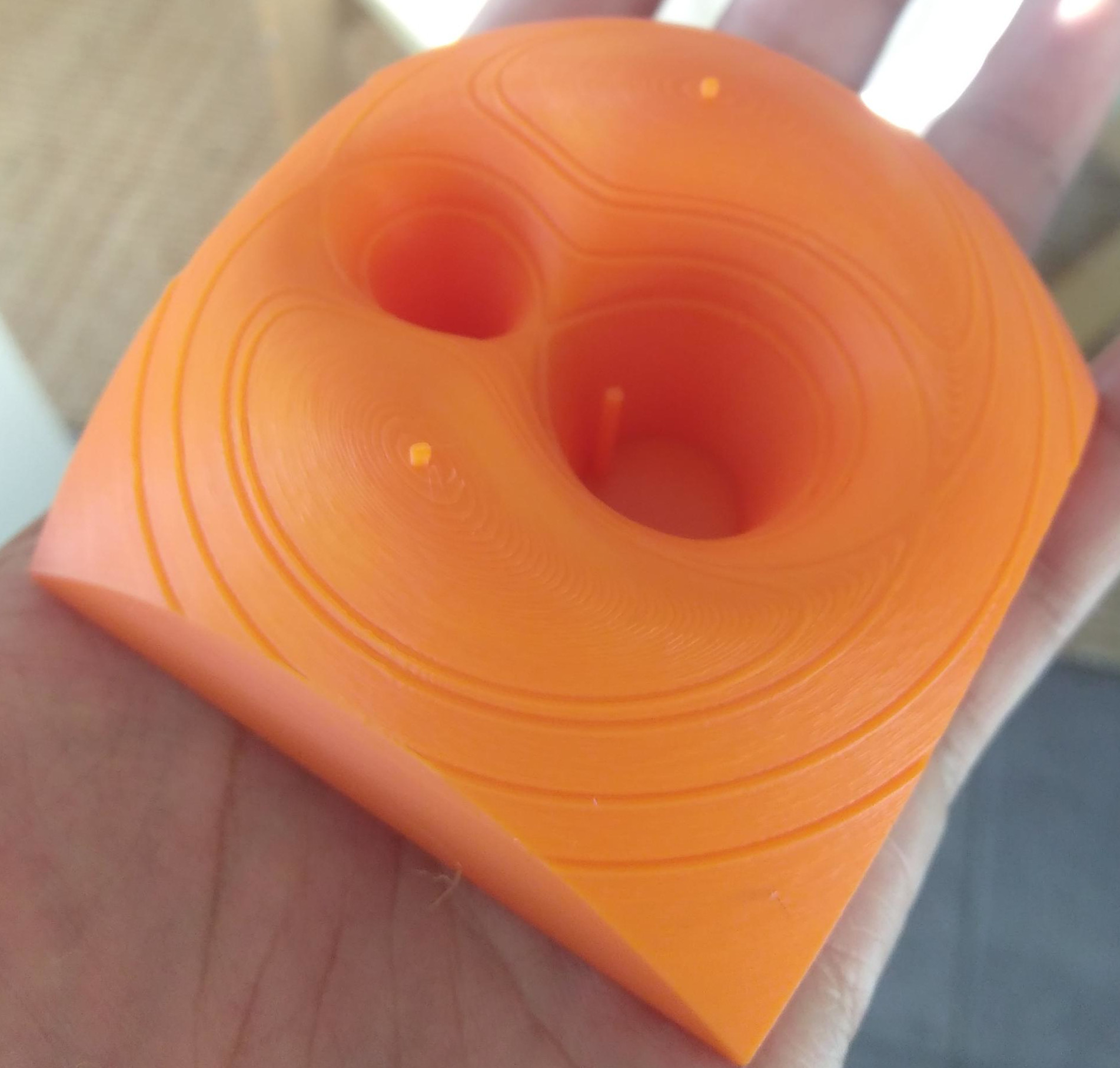
As part of my corona-driven hobbies I ended up getting a 3D printer and doing some 3D modeling. Using the scripting capabilities of blender I made a model of a Roche potential, which is really nice to visualize and teach its properties.

The STL file for printing was produced with blender using the script below. This only produces a base mesh that then needs to be closed down. If you're interested in plotting any type of function with some contour lines, check my github repository blender-function-plot which goes into a bit more detail.

If you want to download and print the STL file check it here. The file there is for a mass ratio of 2. If you're interested in a different mass ratio, let me know!

import bpy
import numpy as np
import bmesh

xvals = np.linspace(-1.5,1.5,400)
yvals = np.linspace(-1.5,1.5,400)

verts = np.zeros((len(xvals),len(yvals),3))

q = 2
x1 = -1/(q+1)
x2 = q/(q+1)

# roche potential
def phi(x,y):
    val = -x2/np.sqrt(np.power(x-x1,2)+np.power(y,2))
    val = val + x1/np.sqrt(np.power(x-x2,2)+np.power(y,2))
    val = val - 0.5*(np.power(x,2) + np.power(y,2))
    return val

# derivative along the line joining both stars
# used to find Lagrangian points
def dphi_dx(x):
    return +x2/np.power(x-x1,2)*np.sign(x-x1) - x1/np.power(x-x2,2)*np.sign(x-x2) - x

# gradient of the potential. This is used to make nice contour lines
def abs_grad_phi(x,y):
    den1 = np.power(np.power(x-x1,2)+np.power(y,2),1.5)
    den2 = np.power(np.power(x-x2,2)+np.power(y,2),1.5)
    dpdx = x2*(x-x1)/den1 - x1*(x-x2)/den2 - x
    dpdy = x2*y/den1 - x1*y/den2 - y
    return np.sqrt(np.power(dpdx,2)+np.power(dpdy,2))

#find L1
x_low = x1*0.99
x_up = x2*0.99
xL1 = 0
while abs(x_low-x_up) > 1e-10:
    xL1 = 0.5*(x_low+x_up)
    if dphi_dx(xL1)>0:
        x_low = xL1
    else:
        x_up = xL1
phiL1 = phi(xL1,0)
print(xL1, phiL1)

#find L3
x_low = -2
x_up = 1.01*x1
xL3 = 0
while abs(x_low-x_up) > 1e-10:
    xL3 = 0.5*(x_low+x_up)
    if dphi_dx(xL3)>0:
        x_low = xL3
    else:
        x_up = xL3
phiL3 = phi(xL3,0)
print(xL3, phiL3)

# find L2
x_low = x2*1.01
x_up = 2
xL2 = 0
while abs(x_low-x_up) > 1e-10:
    xL2 = 0.5*(x_low+x_up)
    if dphi_dx(xL2)>0:
        x_low = xL2
    else:
        x_up = xL2
phiL2 = phi(xL2,0)
print(xL2, phiL2)

#find L4
#L4 and L5 form equilateral triangles with M1 and M2
xL4 = 0.5*(x1+x2)
yL4 = np.sqrt(3)/2*abs(x1-x2)
phiL4 = phi(xL4,yL4)
print(xL4,yL4,phi(xL4,yL4))

# Make one equipotential between L3 and L4
phi_mid = 0.5*(phiL4+phiL3)

phi_cm = phi(0,0)

#create points for mesh
for i, xval in enumerate(xvals):
    for j, yval in enumerate(yvals):
        zval = phi(xval,yval)
        grad = abs_grad_phi(xval,yval)
        if zval > -2.7:
            #this flattens the mesh near equipotentials 
            if (abs(zval-phiL1)) < grad*0.02:
                zval = phiL1
            elif (abs(zval-phiL2)) < grad*0.02:
                zval = phiL2
            elif (abs(zval-phiL3)) < grad*0.02:
                zval = phiL3
            elif (abs(zval-phi_mid)) < grad*0.02:
                zval = phi_mid
            elif (abs(xL4-xval) + abs(yL4-yval) < 0.04):
                zval = phiL4+0.05
            elif (abs(xval) + abs(yval) < 0.04):
                zval = phi_cm+0.4
        zval = max(zval,-2.7)
        verts[i,j] = np.array([xval,yval,zval])
        
mesh = bpy.data.meshes.new("mesh")  # add a new mesh
obj = bpy.data.objects.new("MyObject", mesh)  # add a new object using the mesh

scene = bpy.context.scene
bpy.context.collection.objects.link(obj)
bpy.context.view_layer.objects.active = obj  # set as the active object in the scene
obj.select_set(True)

mesh = bpy.context.object.data
bm = bmesh.new()

vertex_matrix = [[None for x in range(len(xvals))] for y in range(len(yvals))] 

for i, xval in enumerate(xvals):
    for j, yval in enumerate(yvals):
        v = verts[i,j]
        vertex_matrix[i][j] = bm.verts.new(v)  # add a new vert

for i in range(len(xvals)-1):
    for j in range(len(yvals)-1):
        v1 = vertex_matrix[i][j]
        v2 = vertex_matrix[i+1][j]
        v3 = vertex_matrix[i][j+1]
        v4 = vertex_matrix[i+1][j+1]
        face1 = bm.faces.new((v1, v2, v3))
        face2 = bm.faces.new((v2, v3, v4))
        face2.normal_flip()

# make the bmesh the object's mesh
bm.to_mesh(mesh)  
bm.free()  # always do this when finished