Maxilab: Formation of GW sources through Roche lobe overflow

Orbital shrinkage from mass transfer
Save a post-main sequence model
Setup our template for a grid
Let's fill the grid!
Extra work
References

Orbital shrinkage from mass transfer

Under the assumption that mass transfer is extremely inefficient (all mass ejected) and lost material takes away the specific orbital angular momentum of the accretor, the evolution of the orbital separation $a_\mathrm{f}$ can be analitically described. In terms of the final mass ratio $q_\mathrm{f}\equiv m_\mathrm{donor,f}/m_\mathrm{accretor,f}$ and a separation $a_{i}$ at which the system had a mass ratio $q_\mathrm{i}$ we have (Soberman et al. (1988)):

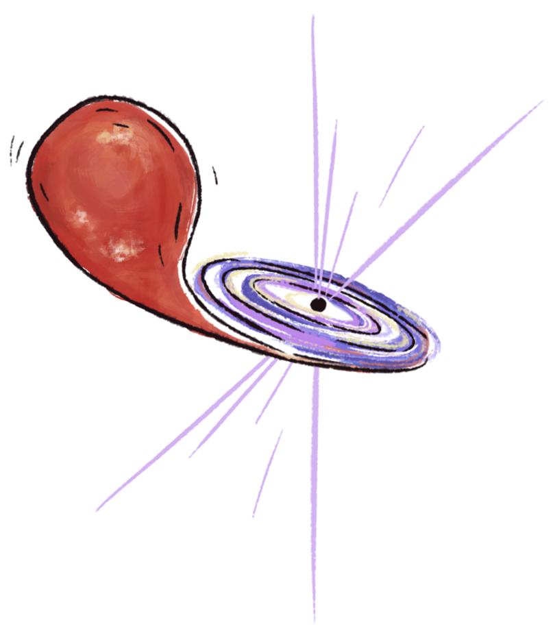
\frac{a_\mathrm{f}}{a_\mathrm{i}}=\left(\frac{q_\mathrm{i}}{q_\mathrm{f}}\right)^2\left(\frac{1+q_\mathrm{i}}{1+q_\mathrm{f}}\right)\exp\left(2[q_\mathrm{f}-q_\mathrm{i}]\right).

The initial and final points needs not refer to that at the onset or end of the mass transfer phase, they can also be any arbitrary point during the process. From that we can estimate how much the orbital separation would change respect to the initial one in terms of the accretor mass and the mass of the companion. In particular, the figure below shows an example of a $30M_\odot$ star being stripped down to $15M_\odot$ by companions of different masses.

$Expected evolution of the orbital separation in terms of initial separation for a $30M_\odot$ donor star being stripped by a companion through fully non-conservative mass transfer (assuming isotropic re-emission from the accretor). Each line is for a different accretor mass.$

Expected evolution of the orbital separation in terms of initial separation for a

30M_\odot

donor star being stripped by a companion through fully non-conservative mass transfer (assuming isotropic re-emission from the accretor). Each line is for a different accretor mass.

So if mass transfer can proceed stably for extreme mass ratios, we could potentially get an extreme reduction in orbital separation! This is particularly interesting in the context of gravitational wave sources (van den Heuvel et al. (2017)), where the time for two point masses to merge depends strongly on the orbital separation. For a circular orbit the merger time is (Peters, P. C. (1964)):

t_\mathrm{merger}=\frac{a^4}{4B},\qquad B\equiv \frac{64G^3}{5c^5}(M_1+M_2)M_1M_2.

Taking arbitrarily high initial mass ratios could in principle lead to arbitrarily small post mass-transfer separations, but there is a competition with mass transfer stability, which we have studied in the previous lab. The purpose of this lab is to study whether or not at the boundary for stability the mass ratio is extreme enough to provide the required shrinkage in orbital separation for gravitational waves to take over. We will consider a $30M_\odot$ donor star with different masses for a black hole companion, and compute a grid of simulations using all the cores at disposition from the attending crowd. Throughout the lab we will make use of mdot_scheme='Kolb'

Save a post-main sequence model

In the interest of time, we will only consider systems which interact after the main sequence. Systems interacting during the main sequence undergo a variety of qualitatively different mass transfer phases, and can be more expensive. Additionally, some of the simplifications we will make below cannot be easily applied for main sequence donors (particularly, we will make use of the helium core mass). Now, if we are just going to consider interaction after the main sequence, it would certainly be useful to avoid repeating the main sequence evoilution every time. So we will first save a model right after the end of the main sequence. We will start with the solution to the previous lab without enhanced angular momentum loss.

Did you have issues finishing minilab2? You can get a working copy of its solution here.

Let us first turn our binary into an effectively single star. To do this we can set in inlist_project

m1 = 30
m2 = 30
initial_period_in_days = 1d5

This will create a wide binary that will not undergo Roche lobe overflow. Set the termination condition in inlist1 to correspond to core-hydrogen depletion:

! stop when the center mass fraction of h1 drops below this limit
xa_central_lower_limit_species(1) = 'h1'
xa_central_lower_limit(1) = 1d-3

And add the following in star_job to create a saved model when the run finishes,

save_model_when_terminate = .true.
save_model_filename = 'TAMS_model.dat'

Run your simulation and see if the TAMS_model.dat file is produced succesfully.

You can also import saved models produced from single star simulations (not using the binary module at all). We did it this way in here to just quickly reuse the work directory we have rather than adjusting a single star work directory.

Setup our template for a grid

Now we will use the saved TAMS model to start up calculations from that point. When loading a saved model, the mass given in m1 or m2 (depending on which model is loaded) is ignored, and instead the mass of the saved model is used.

If you could not create the saved model, you can download a work directory to produce it from here.

Inlist adjustments

Make a new copy of the solution to minilab2 (or download the solution linked above) and copy your saved TAMS file into it. For it to be actually used, include this in the star_job section of inlist1:

load_saved_model = .true.
load_model_filename = 'TAMS_model.dat'

One inconvenience of using a saved model is that it will carry on its model number, so the model number of the star will not be 1 at the start (and it will not match the model number in binary output). Also, the timestep from the saved model will be used in the initial step, which given our very relaxed timestep controls can lead to large overflow in a single step. To fix these two problems, also add the following to star_job in inlist1:

set_initial_dt = .true.
years_for_initial_dt = 1d2
set_initial_model_number = .true.
initial_model_number = 0

The binary module relies in redoing simulation steps with different mass transfer rates until it finds a solution. In case multiple redos happen in a row, a bogus terminating condition can be activated. To prevent this, include this in controls in inlist1:

redo_limit = -1

`run_binary_extras` adjustments

We will need additional information at the end of a run, as well as an additional termination condition. While exploring a grid with multiple physical variations, one thing that can happen is that the binary is too wide to undergo Roche-lobe overflow. So we would like our run to report at the end what was the maximum amount of Roche lobe overflow ( $R/R_\mathrm{Rl}$ ). So to include this information do the following:

In extras_binary_check_model store the value of $R/R_\mathrm{Rl}$ in b% xtra(2) if it exceeds the value of b% xtra(2). By default b% xtra(2) is initiated at zero so in this way you will keep its maximum value.
In extras_binary_after_evolve include a write(*,*) "Check maximum R/R_Rl", b% xtra(2) line to output the maximum value achieved. The extras_binary_after_evolve subroutine is called once the simulation finishes.

The implementation below also includes the previous code to store the time spend in Roche lobe overflow.

!Return either keep_going, retry or terminate
integer function extras_binary_check_model(binary_id)
   type (binary_info), pointer :: b
   integer, intent(in) :: binary_id
   integer :: ierr
   call binary_ptr(binary_id, b, ierr)
   if (ierr /= 0) then ! failure in  binary_ptr
      return
   end if  
   extras_binary_check_model = keep_going

   if (b% r(1) > b% rl(1)) then
      b% xtra(1) = b% xtra(1)+b% time_step
   end if
   write(*,*) "check time", b% xtra(1)

   b% xtra(2) = max(b% r(1)/b% rl(1), b% xtra(2))
  
end function extras_binary_check_model
    
subroutine extras_binary_after_evolve(binary_id, ierr)
   type (binary_info), pointer :: b
   integer, intent(in) :: binary_id
   integer, intent(out) :: ierr
   call binary_ptr(binary_id, b, ierr)
   if (ierr /= 0) then ! failure in  binary_ptr
      return
   end if

   write(*,*) "Check maximum R/R_Rl", b% xtra(2)

end subroutine extras_binary_after_evolve

The other thing we will need to add is a check on overflow. The Kolb scheme allows stars to overflow, with larger mass transfer rates happening at larger overflow. But if the radius of the star exceeds the orbital separation, there's definetely something fishy happening! So go ahead and add another termination condition that checks if the radius of the star exceeds the binary separation (use b% r(1) and b% separation). Remember this can be added in extras_binary_finish_step. Be sure to add a write(*,*) statement saying why the run finished!

! returns either keep_going or terminate.
! note: cannot request retry; extras_check_model can do that.
integer function extras_binary_finish_step(binary_id)
   type (binary_info), pointer :: b
   integer, intent(in) :: binary_id
   integer :: ierr
   real(dp) :: mdot_th, mdot_dyn, avg_rho
   call binary_ptr(binary_id, b, ierr)
   if (ierr /= 0) then ! failure in  binary_ptr
      return
   end if
   extras_binary_finish_step = keep_going

   mdot_th = b% m(1)/(standard_cgrav*(b% m(1))**2/(b% s1% L(1)*b% r(1)))

   avg_rho = b% m(1)/(4d0/3d0*(b% r(1))**3)
   mdot_dyn = b% m(1)/(1/sqrt(standard_cgrav*avg_rho))

   write(*,*) "check mdots", mdot_th/Msun*secyer, mdot_dyn/Msun*secyer
   if (abs(b% mtransfer_rate)>100d0*mdot_th) then
       write(*,*) "Finish simulation due to high mass transfer rate"
       extras_binary_finish_step = terminate
   end if

   if (b% r(1) > b% separation) then
       write(*,*) "Finish simulation due to radius exceeding separation"
       extras_binary_finish_step = terminate
   end if

end function extras_binary_finish_step

Approximating the final state of the binary

Now, rather than modeling the system all the way to helium depletion, we will make some big assumptions for its final state when a binary black hole can form. This will allow us to only model a fraction of its evolution which is useful to explore a large input parameter space.

We will assume that after the donor reaches $20M_\odot$ , mass transfer will proceed succesfully until the star is stripped down to its helium core.
The final separation after mass transfer will be computed using Equation (1).
We will assume that after stripping, mass loss is negligible and the star will form a black hole with no mass loss at all (direct collapse while ignoring any neutrino losses). This means we also take the separation after mass transfer to be the separation when the binary black hole forms. Using than information we will compute the merger time with Equation (2).

To include a termination condition based in reaching a minimum mass limit, you can use star_mass_min_limit = 20d0 in the controls section of inlist1.

The information on the helium core mass is stored in the star_info variable he_core_mass. In run_binary_extras you can access it with b% s1% he_core_mass. Beware that this is not in grams but in $M_\odot$ units! Now, we are not interested in you spending too much time just typing equations, so we provide you here the solution right away. The following is the final version of extras_binary_after_evolve, be sure to check it and understand what it is doing (it includes the reporting of maximum overflow implemented previously).

subroutine extras_binary_after_evolve(binary_id, ierr)
   type (binary_info), pointer :: b
   integer, intent(in) :: binary_id
   integer, intent(out) :: ierr
   real(dp) :: m1f, m2f, qi, qf, ai, af, Bmerge, tmerge
   call binary_ptr(binary_id, b, ierr)
   if (ierr /= 0) then ! failure in  binary_ptr
      return
   end if

   qi = b% m(1)/b% m(2)

   m1f = b% s1% he_core_mass*Msun ! assume stripping down to the helium core
   m2f = b% m(2) ! assume no further accretion
   qf = (b% s1% he_core_mass*Msun)/b% m(2)

   ai = b% separation
   af = ai*(qi/qf)**2*((1+qi)/(1+qf))*exp(2*(qf-qi))

   Bmerge = 64d0/5d0*standard_cgrav**3/clight**5*(m1f+m2f)*m1f*m2f
   tmerge = af**4/(4d0*Bmerge)

   write(*,*) "Merger time in Gigayears", tmerge/secyer/1e9
   write(*,*) "Check maximum R/R_Rl", b% xtra(2)

end subroutine extras_binary_after_evolve

Let's fill the grid!

Now that everything is ready, let's go ahead and start running simulations! This is a group effort for all the participants, so we will need to coordinate a bit. We will fill the results of our simulations in this google spreadsheet.

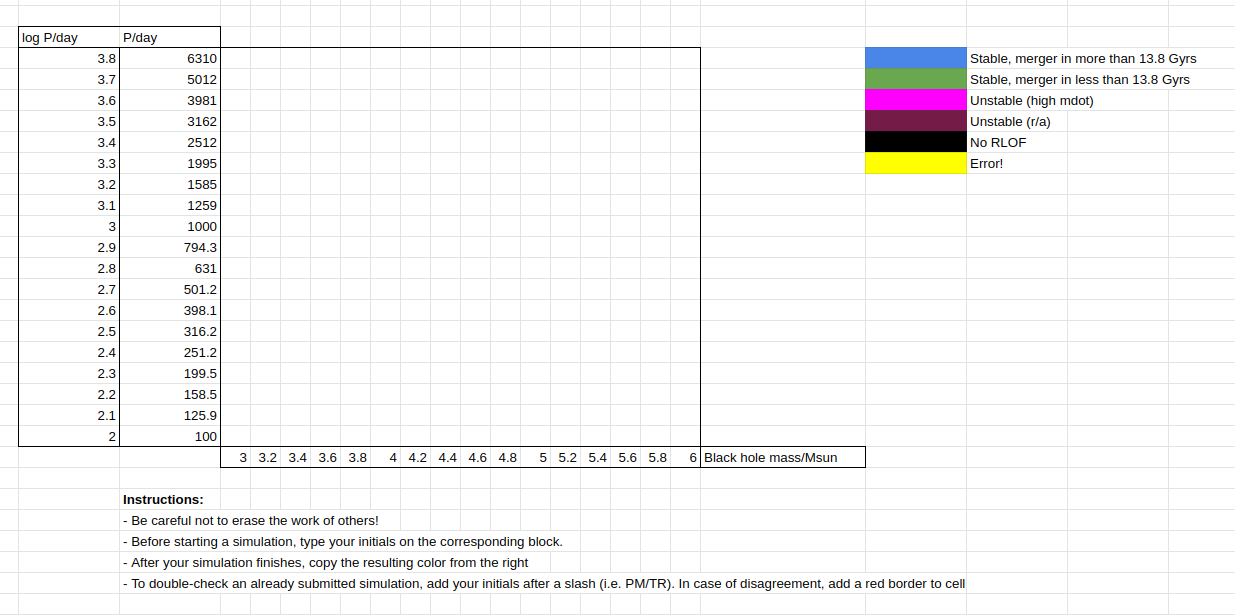
Screenshot of the google sheet we will fill.

If you are having problems setting up the template for the grid simulation, you can download it here.

The initial parameters we will vary are the initial period (separated in equal intervals of $\log P$ of $0.1$ dex) and mass of the companion black hole (covering between $3M_\odot$ and $6M_\odot$ ). The online sheet also lists the value of the period in days rather than $\log P$ , for easy inclusion in your inlist. It is useful to repeat simulations to validate the results from others, but first start by trying to populate the grid and finding the boundaries between different outcomes. The potential outcomes we consider here are:

Mass transfer is stable (reaches star_min_mass_limit) but the resulting binary black hole takes more than $13.8$ Gyr to merge.
Mass transfer is stable (reaches star_min_mass_limit) but the resulting binary black hole takes less than $13.8$ Gyr to merge. These are the ones we are looking for!
System is unstable due to reaching the limit given by $100\times\dot{M}_\mathrm{thermal}$ .
System is unstable due to the donor expanding to a radius larger than the binary separation.
System does not interact (orbit is too wide).
A numerical error happens (cross our fingers that these are minimal).

As the plot begins to take shape, discuss with your tablemates what different regions can be seen, and what is the reason for the different trends that appear.

Extra work

And in case you're already saturated of filling out the simulation grid, how about removing the star_mass_min_limit terminating condition and repeating some of the runs that were marked as resulting in a gravitational-wave driven merger within $13.8$ Gyr. How close is the final system to the one with the approximations used?

References

Peters, P. C., Physical Review, vol. 136, Issue 4B, pp. 1224-1232
Soberman, G. E.; Phinney, E. S.; van den Heuvel, E. P. J., Astronomy and Astrophysics, v.327, p.620-635
van den Heuvel, E. P. J.; Portegies Zwart, S. F.; de Mink, S. E., Monthly Notices of the Royal Astronomical Society, Volume 471, Issue 4, p.4256-4264

CC BY-SA 4.0 Pablo Marchant. Last modified: August 09, 2022. Website built with Franklin.jl and the Julia programming language.