© Pablo Marchant.
© Pablo Marchant.
In the first minilab of this session we will work on constructing a basic setup to model a single-degenerate binary system consisting of a black hole and a star. We will also study how different prescriptions to compute mass transfer rates can impact observable properties of the system. The structure of the stellar component in such a simulation is modelled by MESA, while the black hole is only modeled as a sink. In particular we will be studying cases in which the luminosity released by the compact object from accretion is much larger than its Eddington luminosity,
where is the mass of the black hole, and is the opacity of accreted material. A black hole accreting through a disk is expected to have a luminosity proportional to its accretion rate, , where depends on the spin of the black hole. Assuming only electron-scattering opacity, , one can then determine at which mass transfer rate the resulting luminosity would reach
In our MESA simulations we will consider that all mass transfer in excess of is ejected from the vicinity of the black hole carrying its specific orbital angular momentum.
binary work directoryWe will start by copying up an example working repository from MESA. You can do this from your terminal by running the following command from the directory where you want to setup this work directory
cp -r $MESA_DIR/binary/work template
cd template
tree
the tree command shows all files contained within the current folder, its output should look like this:
.
├── clean
├── inlist
├── inlist1
├── inlist2
├── inlist_project
├── make
│   └── makefile
├── mk
├── re
├── rn
└── src
    ├── binary_run.f90
    ├── run_binary_extras.f90
└── run_star_extras.f90tree command is not available in your system, you can also use ls -lh * to see all files within the work folder.As you can see, the structure of a binary work folder is similar to that of a star.
binary work folderThe file inlist_project now contains options relevant to the binary system rather than each component. inlist1 and inlist2 are the inlists that are used for each component, and contain the same options you can use with single star simulations. Doing a sneak peek into inlist_project one finds the following:
&binary_job

   inlist_names(1) = 'inlist1'
   inlist_names(2) = 'inlist2'

   evolve_both_stars = .false.

/ ! end of binary_job namelist

&binary_controls

   m1 = 1.0d0  ! donor mass in Msun
   m2 = 1.4d0 ! companion mass in Msun
   initial_period_in_days = 2d0

   !transfer efficiency controls
   limit_retention_by_mdot_edd = .true.

   max_tries_to_achieve = 20

/ ! end of binary_controls namelist
You can check all options available in the files
$MESA_DIR/binary/defaults/binary_job.defaults
$MESA_DIR/binary/defaults/binary_controls.defaults
In particular, the options included in inlist_project serve the following purpose
inlist_names(*): The inlists of each star do not have hard-coded names and can be modified with this.
evolve_both_stars: If true, MESA will model both stars, otherwise star 2 will be set to a point mass. In this case inlist2 is ignored.
m1, m2 and initial_period_in_days: The initial mass and period of the binary system. Default for eccentricity is zero.
limit_retention_by_mdot: If true, then the accretion rate is limited to . Excess transferred mass is ejected with the specific angular momentum of the point mass.
max_tries_to_achieve: Numerical option for the implicit mass transfer solver. This provides the number of iterations the solver will do.
As you can see our simulation is already set up to model one of the components as a point mass with Eddington limited accretion
One last important thing to note is that in inlist1 the LOGS directory is modified, in particular, inlist1 has:
&controls

      extra_terminal_output_file = 'log1'
      log_directory = 'LOGS1'

      ...

/ ! end of controls namelist
In cases where both stars are modeled this prevents a collision of output within the same directory.
run_binary_extras.f90 and run_star_extras.f90Another difference from a star work folder is the run_binary_extras.f90 file in src. This file offers similar functionality to run_star_extras.f90, allowing for the inclusion of custom output, modified physics and termination conditions among others. For example, additional output from the binary system can be included through the following subroutines:
integer function how_many_extra_binary_history_columns(binary_id)
   use binary_def, only: binary_info
   integer, intent(in) :: binary_id
   how_many_extra_binary_history_columns = 0
end function how_many_extra_binary_history_columns

subroutine data_for_extra_binary_history_columns(binary_id, n, names, vals, ierr)
   type (binary_info), pointer :: b
   integer, intent(in) :: binary_id
   integer, intent(in) :: n
   character (len=maxlen_binary_history_column_name) :: names(n)
   real(dp) :: vals(n)
   integer, intent(out) :: ierr
   ierr = 0
   call binary_ptr(binary_id, b, ierr)
   if (ierr /= 0) then
      write(*,*) 'failed in binary_ptr'
      return
   end if

end subroutine data_for_extra_binary_history_columns
As there is a star_info type to contain information on a stellar model, there is a binary_info type that contains information specific to the binary system, such as its orbital period. The information contained within this type can be checked in the file $MESA_DIR/binary/public/binary_data.inc. Some examples of useful values are:
b% mtransfer_rate: The mass transfer rate from the donor to the accretor. Not all mass needs to be accreted though, and in particular we will study cases where mass transfer is very inneficient.
b% s1 and b% s2: The star_info instances for each component. If only modeling one component, b% s2 will not be defined.
b% m(1) and b% m(2): The mass of each component in grams.
b% xtra(:): Allows to store information. For instance, b% xtra(1) could be used to store the time during which a specific condition in the simulation has been met. The benefit of using this over a global variable in run_binary_extras.f90 is that MESA will automatically take care of it during restarts of simulations.
binary modelTo run this work folder of binary one proceeds in the same way as in star:
./mk
./rn | tee out.txt
The ./mk command is only needed when modifying the run_*_extras files, modification of inlist files does not require recompilation. The tee command is just a convenient way to store the terminal output in a file while still displaying it in the terminal. Try running your work folder for a few (at least 50) steps and then stop the simulation by pressing ctrl+c (or however that is done in a mac, cmd+c?). First thing you will notice is a significant amount of additional output, including both information for the star in the model as well as the binary system:
__________________________________________________________________________________________________________________________________________________

       step    lg_Tmax     Teff     lg_LH      lg_Lnuc     Mass       H_rich     H_cntr     N_cntr     Y_surf   eta_cntr   zones  retry
  lg_dt_yrs    lg_Tcntr    lg_R     lg_L3a     lg_Lneu     lg_Mdot    He_core    He_cntr    O_cntr     Z_surf   gam_cntr   iters
    age_yrs    lg_Dcntr    lg_L     lg_LZ      lg_Lphoto   lg_Dsurf   CO_core    C_cntr     Ne_cntr    Z_cntr   v_div_cs       dt_limit
__________________________________________________________________________________________________________________________________________________

         50   7.147318   5671.430  -0.103097  -0.103097   1.000000   1.000000   0.600603   0.005051   0.280000  -1.649360    791      0
 7.8169E+00   7.147318  -0.036243 -45.850679  -1.763204 -99.000000   0.000000   0.378831   0.009337   0.020000   0.093456     10
 1.3577E+09   1.982613  -0.103022 -99.000000 -99.000000  -6.735325   0.000000   0.000016   0.002085   0.020566  0.000E+00        b_jorb
__________________________________________________________________________________________________________________________________________________

binary_step      M1+M2      separ       Porb          e      M2/M1       pm_i    donor_i    dot_Mmt        eff       Jorb      dot_J    dot_Jmb
      lg_dt         M1         R1         P1      dot_e      vorb1        RL1    Rl_gap1     dot_M1   dot_Medd      spin1    dot_Jgr    dot_Jls
     age_yr         M2         R2         P2       Eorb      vorb2        RL2    Rl_gap2     dot_M2      L_acc      spin2    dot_Jml  rlo_iters
__________________________________________________________________________________________________________________________________________________

bin      50   2.400000   8.627141   1.894689  0.000E+00   1.400000          2          1  0.000E+00   1.000000  1.604E+52 -7.975E+33 -7.720E+33
   7.816944   1.000000   0.919935   0.000000  0.000E+00 134.379739   3.021149 -6.955E-01  0.000E+00  6.357E-08  0.000E+00 -2.547E+32  0.000E+00
 1.3577E+09   1.400000   0.000000   0.000000 -3.078E+47  95.985528   3.522940 -1.000E+00  0.000E+00  0.000E+00  0.000E+00  0.000E+00          1
The file structure also shows some small differences compared to a star simulation, which you can check with the tree command
.
├── binary
├── binary_history.data
├── clean
├── inlist
├── inlist1
├── inlist2
├── inlist_project
├── log1
├── LOGS1
│   ├── history.data
│   ├── pgstar.dat
│   ├── profile1.data
│   ├── profile2.data
│   └── profiles.index
├── make
│   ├── binary_run.o
│   ├── makefile
│   ├── run_binary_extras.mod
│   ├── run_binary_extras.o
│   ├── run_binary_extras.smod
│   ├── run_binary.mod
│   ├── run_binary.o
│   ├── run_star_extras.mod
│   ├── run_star_extras.o
│   └── run_star_extras.smod
├── mk
├── out.txt
├── photos
│   ├── 1_x050
│   └── b_x050
├── re
├── rn
└── src
    ├── binary_run.f90
    ├── run_binary_extras.f90
    └── run_star_extras.f90
Particularly important in here is the binary_history.data file, which contains information from the binary model in a similar format to history.data.
1                                2                                3                                4                                5                                6                                7                                8
                  version_number                 initial_don_mass                 initial_acc_mass              initial_period_days                         compiler                            build                 MESA_SDK_version                             date
                      "r22.05.1"          1.0000000000000000E+000          1.3999999999999999E+000          2.0000000000000000E+000                       "gfortran"                         "10.2.0"            "x86_64-linux-21.4.1"                       "20220623"

                               1                                2                                3                                4                                5                                6                                7                                8                                9                               10                               11                               12                               13                               14                               15                               16                               17                               18                               19                               20                               21                               22                               23                               24                               25                               26                               27                               28                               29                               30                               31
                    model_number                              age                      period_days                binary_separation                          v_orb_1                          v_orb_2                             rl_1                             rl_2           rl_relative_overflow_1           rl_relative_overflow_2                      star_1_mass                      star_2_mass                lg_mtransfer_rate                   lg_mstar_dot_1                   lg_mstar_dot_2                 lg_system_mdot_1                 lg_system_mdot_2                   lg_wind_mdot_1                   lg_wind_mdot_2              fixed_xfer_fraction                eff_xfer_fraction                            J_orb                             Jdot                          jdot_mb                          jdot_gr                          jdot_ml                          jdot_ls                jdot_missing_wind                       extra_jdot                      donor_index                 point_mass_index
                               5          7.4416000000000000E+005          1.9999980489355869E+000          8.9439202746766693E+000          1.3197852504643137E+002          9.4270375033165308E+001          3.1320820960887494E+000          3.6522989775229004E+000         -7.1732731040477715E-001         -1.0000000000000000E+000          1.0000000000000000E+000          1.3999999999999997E+000         -9.8999999999999986E+001         -9.8999999999999986E+001         -9.8999999999999986E+001         -9.8999999999999986E+001         -9.8999999999999986E+001         -9.8999999999999986E+001         -9.8999999999999986E+001          1.0000000000000000E+000          1.0000000000000000E+000          1.6328981745087756E+052         -2.2610479693263478E+032          0.0000000000000000E+000         -2.2610479693263478E+032          0.0000000000000000E+000          0.0000000000000000E+000          0.0000000000000000E+000          0.0000000000000000E+000                                1                                2
                              10          2.5958682111999998E+006          1.9999931940509912E+000          8.9439058007564380E+000          1.3197863183679308E+002          9.4270451311995089E+001          3.1320770274493812E+000          3.6522930670180624E+000         -7.1846295523455295E-001         -1.0000000000000000E+000          1.0000000000000000E+000          1.3999999999999997E+000         -9.8999999999999986E+001         -9.8999999999999986E+001         -9.8999999999999986E+001         -9.8999999999999986E+001         -9.8999999999999986E+001         -9.8999999999999986E+001         -9.8999999999999986E+001          1.0000000000000000E+000          1.0000000000000000E+000          1.6328968532510521E+052         -2.2610586415692399E+032          0.0000000000000000E+000         -2.2610586415692399E+032          0.0000000000000000E+000          0.0000000000000000E+000          0.0000000000000000E+000          0.0000000000000000E+000                                1                                2
                              15          7.2035107872931827E+006          1.9999811134701584E+000          8.9438697847386237E+000          1.3197889756852246E+002          9.4270641120373199E+001          3.1320644149571950E+000          3.6522783596793333E+000         -7.1804224478624690E-001         -1.0000000000000000E+000          1.0000000000000000E+000          1.3999999999999997E+000         -9.8999999999999986E+001         -9.8999999999999986E+001         -9.8999999999999986E+001         -9.8999999999999986E+001         -9.8999999999999986E+001         -9.8999999999999986E+001         -9.8999999999999986E+001          1.0000000000000000E+000          1.0000000000000000E+000          1.6328935655095063E+052         -2.2610851979732856E+032          0.0000000000000000E+000         -2.2610851979732856E+032          0.0000000000000000E+000          0.0000000000000000E+000          0.0000000000000000E+000          0.0000000000000000E+000                                1                                2
                              20          1.8668799962237373E+007          1.9999510526586048E+000          8.9437801636730807E+000          1.3197955881352075E+002          9.4271113438229136E+001          3.1320330304494854E+000          3.6522417624248869E+000         -7.1682239453910634E-001         -1.0000000000000000E+000          1.0000000000000000E+000          1.3999999999999997E+000         -9.8999999999999986E+001         -9.8999999999999986E+001         -9.8999999999999986E+001         -9.8999999999999986E+001         -9.8999999999999986E+001         -9.8999999999999986E+001         -9.8999999999999986E+001          1.0000000000000000E+000          1.0000000000000000E+000          1.6328853843736342E+052         -2.2611512815823777E+032          0.0000000000000000E+000         -2.2611512815823777E+032          0.0000000000000000E+000          0.0000000000000000E+000          0.0000000000000000E+000          0.0000000000000000E+000                                1                                2
These data are also copied into the single star history file, LOGS1/history.data. This is just an internal workaround in the code to allow for information from the binary system to be included in pgstar plots. To change the information contained in binary_history.data, you can copy the file $MESA_DIR/binary/defaults/binary_history_columns.list to your work folder and comment/uncomment the necessary fields. Alternatively, new fields can be added with the subroutines of run_binary_extras that where mentioned previously.
Also from the files shown above, you can see that the photos, which are needed to restart simulations, are stored differently from star. For each saved timestep a photo is saved containing the information of each star modeled, as well as one from the binary system. To restart a simulation from step 50, you can then do.
./re x050 | tee outre.txtNext we will perform some adjustments to the template. A significant number of these are meant to make the simulation faster in order to be efficiently computed in the duration of this lab.
@binary_controls section of inlist_projectWe will first consider a system of a massive star with a black hole companion in an orbit wide enough for interaction to happen after the main-sequence. For this we modify the values of m1, m2 and initial_period_in_days:
m1 = 30d0  ! donor mass in Msun
m2 = 20d0 ! companion mass in Msun
initial_period_in_days = 50d0
By default MESA also includes the effect of magnetic braking for angular momentum loss. This implementation is meant for late type stars and should be removed when working with massive binaries, for that purpose you can include:
do_jdot_mb = .false.Finally, to run the simulation faster we will relax multiple timestepping controls of the binary module by including:
! relax timestep controls
fm = 0.1d0
fa = 0.02d0
fa_hard = 0.04d0
fr = 0.5d0
fj = 0.01d0
fj_hard = 0.02d0
The exact purpose of each of these controls can be checked in the defaults file mentioned previously. Contrary to star there is not a single time_delta_coeff control to easily scale all timesteps, but this will be provided at some point in future versions.
@controls section of inlist1Next we will modify the settings for the star that will be modeled. We will start by including wind mass loss, which is an important ingredient while modeling massive stars:
! mass loss options
cool_wind_full_on_T = 0.8d4
hot_wind_full_on_T = 1.2d4
cool_wind_RGB_scheme = 'Dutch'
cool_wind_AGB_scheme = 'Dutch'
hot_wind_scheme = 'Dutch'
Dutch_wind_lowT_scheme = 'de Jager'
Dutch_scaling_factor = 1.0d0
Here we have included the Dutch prescription of mass loss that is coded in MESA. Beware that this prescription is just a combination of various published prescriptions that are designed for different stars. If you ever use the Dutch prescription in a published paper be aware that it is not ok to describe your mass loss as "the Dutch scheme from MESA", you need to give proper credit to the individual prescriptions it uses. In particular for the above options winds will be computed as a combination of the prescriptions from de Jager et al. (1988), Nugis & Lamers et al. (2000) and Vink et al. (2001).
Massive stars are also expected to have strong overshooting from their convective cores. We include some options for this, as well as to use the Ledoux criterion to determine convective boundaries (the amount of overshooting chosen follows the calibration of Brott et al. (2011) for core hydrogen burning, while for core helium burning we use a bit of exponential overshooting):
! we use step overshooting
overshoot_scheme(1) = 'step'
overshoot_zone_type(1) = 'burn_H'
overshoot_zone_loc(1) = 'core'
overshoot_bdy_loc(1) = 'top'
overshoot_f(1) = 0.345
overshoot_f0(1) = 0.01

! a bit of exponential overshooting for convective core during He burn
overshoot_scheme(2) = 'exponential'
overshoot_zone_type(2) = 'burn_He'
overshoot_zone_loc(2) = 'core'
overshoot_bdy_loc(2) = 'top'
overshoot_f(2) = 0.01
overshoot_f0(2) = 0.005

use_ledoux_criterion = .true.
alpha_semiconvection = 1d0
As modeling evolution all the way to core collapse is expensive, we will only follow it until core helium depletion:
! stop when the center mass fraction of h1 drops below this limit
xa_central_lower_limit_species(1) = 'he4'
xa_central_lower_limit(1) = 1d-3
For the simulations we will significantly reduce the resolution and reduce the tolerance of the solver. This is only meant to make these labs faster and reduce the time you spend simply watching a screen, doing this for a simulation meant for publication is not advised.
! reduce resolution and solver tolerance to make runs faster
mesh_delta_coeff = 3d0
time_delta_coeff = 3d0
varcontrol_target = 1d-2
use_gold2_tolerances = .false.
use_gold_tolerances = .true.
And we will also include some adjustments to the solver. These options can reduce changes in individual solver iterations and help it find solutions, unlike the relaxed tolerance from the options above these options can be a good option to work out solver issues in publication-quality runs:
! Use scaled corrections to aid the solver
scale_max_correction = 0.03d0
ignore_min_corr_coeff_for_scale_max_correction = .true.
ignore_species_in_max_correction = .true.
scale_max_correction_for_negative_surf_lum = .true.
Finally, we also include the following options
use_superad_reduction = .true.
eps_mdot_leak_frac_factor = 0d0
The first option activates an implicit method to enhance energy transport in regions near the Eddington limit of the star. It can help simulations towards the end of mass transfer, but should be thought of more as stellar engineering than an actual physical model. The second one removes a correction to the energy equation during mass transfer. Although this ignores a physical effect, its implementation can make our simulations unstable so for simplicity we will ignore it.
@pgstar section of inlist1For pgstar here is a pre-made grid that will show most of what you need. You can also include pause_before_terminate = .true. in @star_job so that your pgstar plot does not vanish at the end of the run. Every 100 steps the output will be saved in the folder png1. Another useful pgstar option to add in @star_job is save_pgstar_files_when_terminate = .true.. This will ensure the pgstar output is saved at the very last step.
pgstar_interval = 1

pgstar_age_disp = 2.5
pgstar_model_disp = 2.5

!### scale for axis labels
pgstar_xaxis_label_scale = 1.3
pgstar_left_yaxis_label_scale = 1.3
pgstar_right_yaxis_label_scale = 1.3

Grid2_win_flag = .true.

Grid2_win_width = 15
Grid2_win_aspect_ratio = 0.65 ! aspect_ratio = height/width

Grid2_plot_name(4) = 'Mixing'

Grid2_num_cols = 7 ! divide plotting region into this many equal width cols
Grid2_num_rows = 8 ! divide plotting region into this many equal height rows
Grid2_num_plots = 6 ! <= 10

Grid2_plot_name(1) = 'TRho_Profile'
Grid2_plot_row(1) = 1 ! number from 1 at top
Grid2_plot_rowspan(1) = 3 ! plot spans this number of rows
Grid2_plot_col(1) =  1 ! number from 1 at left
Grid2_plot_colspan(1) = 2 ! plot spans this number of columns
Grid2_plot_pad_left(1) = -0.05 ! fraction of full window width for padding on left
Grid2_plot_pad_right(1) = 0.01 ! fraction of full window width for padding on right
Grid2_plot_pad_top(1) = 0.00 ! fraction of full window height for padding at top
Grid2_plot_pad_bot(1) = 0.05 ! fraction of full window height for padding at bottom
Grid2_txt_scale_factor(1) = 0.65 ! multiply txt_scale for subplot by this


Grid2_plot_name(5) = 'Kipp'
Grid2_plot_row(5) = 4 ! number from 1 at top
Grid2_plot_rowspan(5) = 3 ! plot spans this number of rows
Grid2_plot_col(5) =  1 ! number from 1 at left
Grid2_plot_colspan(5) = 2 ! plot spans this number of columns
Grid2_plot_pad_left(5) = -0.05 ! fraction of full window width for padding on left
Grid2_plot_pad_right(5) = 0.01 ! fraction of full window width for padding on right
Grid2_plot_pad_top(5) = 0.03 ! fraction of full window height for padding at top
Grid2_plot_pad_bot(5) = 0.0 ! fraction of full window height for padding at bottom
Grid2_txt_scale_factor(5) = 0.65 ! multiply txt_scale for subplot by this
Kipp_title = ''
Kipp_show_mass_boundaries = .true.

Grid2_plot_name(6) = 'HR'
HR_title = ''
Grid2_plot_row(6) = 7 ! number from 1 at top
Grid2_plot_rowspan(6) = 2 ! plot spans this number of rows
Grid2_plot_col(6) =  6 ! number from 1 at left
Grid2_plot_colspan(6) = 2 ! plot spans this number of columns

Grid2_plot_pad_left(6) = 0.05 ! fraction of full window width for padding on left
Grid2_plot_pad_right(6) = -0.01 ! fraction of full window width for padding on right
Grid2_plot_pad_top(6) = 0.0 ! fraction of full window height for padding at top
Grid2_plot_pad_bot(6) = 0.0 ! fraction of full window height for padding at bottom
Grid2_txt_scale_factor(6) = 0.65 ! multiply txt_scale for subplot by this

History_Panels1_title = ''
History_Panels1_num_panels = 3

History_Panels1_xaxis_name='model_number'
History_Panels1_max_width = -1 ! only used if > 0.  causes xmin to move with xmax.

History_Panels1_yaxis_name(1) = 'period_days'
History_Panels1_other_yaxis_name(1) = ''
History_Panels1_yaxis_log(1) = .true.
History_Panels1_yaxis_reversed(1) = .false.
History_Panels1_ymin(1) = -101d0 ! only used if /= -101d0
History_Panels1_ymax(1) = -101d0 ! only used if /= -101d0
!History_Panels1_dymin(1) = 0.1

History_Panels1_yaxis_name(2) = 'lg_mtransfer_rate' !
History_Panels1_yaxis_reversed(2) = .false.
History_Panels1_ymin(2) = -8d0 ! only used if /= -101d0
History_Panels1_ymax(2) = -1d0 ! only used if /= -101d0
History_Panels1_dymin(2) = 1

History_Panels1_other_yaxis_name(2) = 'log_abs_mdot'
History_Panels1_other_yaxis_reversed(2) = .false.
History_Panels1_other_ymin(2) = -8d0 ! only used if /= -101d0
History_Panels1_other_ymax(2) = -1d0 ! only used if /= -101d0
History_Panels1_other_dymin(2) = 1

History_Panels1_yaxis_name(3) = 'rl_relative_overflow_1'
History_Panels1_other_yaxis_name(3) = ''
History_Panels1_yaxis_reversed(3) = .false.

Grid2_plot_name(2) = 'Text_Summary1'
Grid2_plot_row(2) = 7 ! number from 1 at top
Grid2_plot_rowspan(2) = 2 ! plot spans this number of rows
Grid2_plot_col(2) = 1 ! number from 1 at left
Grid2_plot_colspan(2) = 4 ! plot spans this number of columns
Grid2_plot_pad_left(2) = -0.08 ! fraction of full window width for padding on left
Grid2_plot_pad_right(2) = -0.10 ! fraction of full window width for padding on right
Grid2_plot_pad_top(2) = 0.08 ! fraction of full window height for padding at top
Grid2_plot_pad_bot(2) = -0.04 ! fraction of full window height for padding at bottom
Grid2_txt_scale_factor(2) = 0.19 ! multiply txt_scale for subplot by this
Text_Summary1_name(7,1) = 'period_days'
Text_Summary1_name(8,1) = 'star_2_mass'

Grid2_plot_name(3) = 'Profile_Panels3'
Profile_Panels3_title = 'Abundance-Power-Mixing'
Profile_Panels3_num_panels = 3
Profile_Panels3_yaxis_name(1) = 'Abundance'
Profile_Panels3_yaxis_name(2) = 'Power'
Profile_Panels3_yaxis_name(3) = 'Mixing'

Profile_Panels3_xaxis_name = 'mass'
Profile_Panels3_xaxis_reversed = .false.

Grid2_plot_row(3) = 1 ! number from 1 at top
Grid2_plot_rowspan(3) = 6 ! plot spans this number of rows
Grid2_plot_col(3) = 3 ! plot spans this number of columns
Grid2_plot_colspan(3) = 3 ! plot spans this number of columns

Grid2_plot_pad_left(3) = 0.09 ! fraction of full window width for padding on left
Grid2_plot_pad_right(3) = 0.07 ! fraction of full window width for padding on right
Grid2_plot_pad_top(3) = 0.0 ! fraction of full window height for padding at top
Grid2_plot_pad_bot(3) = 0.0 ! fraction of full window height for padding at bottom
Grid2_txt_scale_factor(3) = 0.65 ! multiply txt_scale for subplot by this

Grid2_plot_name(4) = 'History_Panels1'
Grid2_plot_row(4) = 1 ! number from 1 at top
Grid2_plot_rowspan(4) = 6 ! plot spans this number of rows
Grid2_plot_col(4) =  6 ! number from 1 at left
Grid2_plot_colspan(4) = 2 ! plot spans this number of columns
Grid2_plot_pad_left(4) = 0.05 ! fraction of full window width for padding on left
Grid2_plot_pad_right(4) = 0.03 ! fraction of full window width for padding on right
Grid2_plot_pad_top(4) = 0.0 ! fraction of full window height for padding at top
Grid2_plot_pad_bot(4) = 0.07 ! fraction of full window height for padding at bottom
Grid2_txt_scale_factor(4) = 0.65 ! multiply txt_scale for subplot by this

Grid2_file_flag = .true.
Grid2_file_dir = 'png1'
Grid2_file_prefix = 'grid_'
Grid2_file_interval = 100 ! 1 ! output when mod(model_number,Grid2_file_interval)==0
Grid2_file_width = -1 ! negative means use same value as for window
Grid2_file_aspect_ratio = -1 ! negative means use same value as for window
In order for the Kippenhahn diagram to show up in the simulation one needs to add additional input to the history file. For this purpose, copy the history_columns.list file into your work directory:
cp $MESA_DIR/star/defaults/history_columns.list .In the file look for the mixing_regions option, and above it add a line saying mixing_regions 10. Specifically, the file will originally look like this:
! you might want to get a more complete list of mixing regions by using the following

!mixing_regions <integer> ! note: this includes regions where the mixing type is no_mixing.

   ! the <integer> is the number of regions to report
   ! there will be 2*<integer> columns for this in the log file, 2 for each region.
   ! the first column for a region gives the mixing type as defined in const/public/const_def.f90.
and after editing it will look like this:
! you might want to get a more complete list of mixing regions by using the following
mixing_regions 10
!mixing_regions <integer> ! note: this includes regions where the mixing type is no_mixing.

   ! the <integer> is the number of regions to report
   ! there will be 2*<integer> columns for this in the log file, 2 for each region.
! the first column for a region gives the mixing type as defined in const/public/const_def.f90.After all this work you should be all set to go. You can test your setup by running
./rn | tee out.txtwhich should give you a nice pgstar window that looks like the following after a bit of evolution:
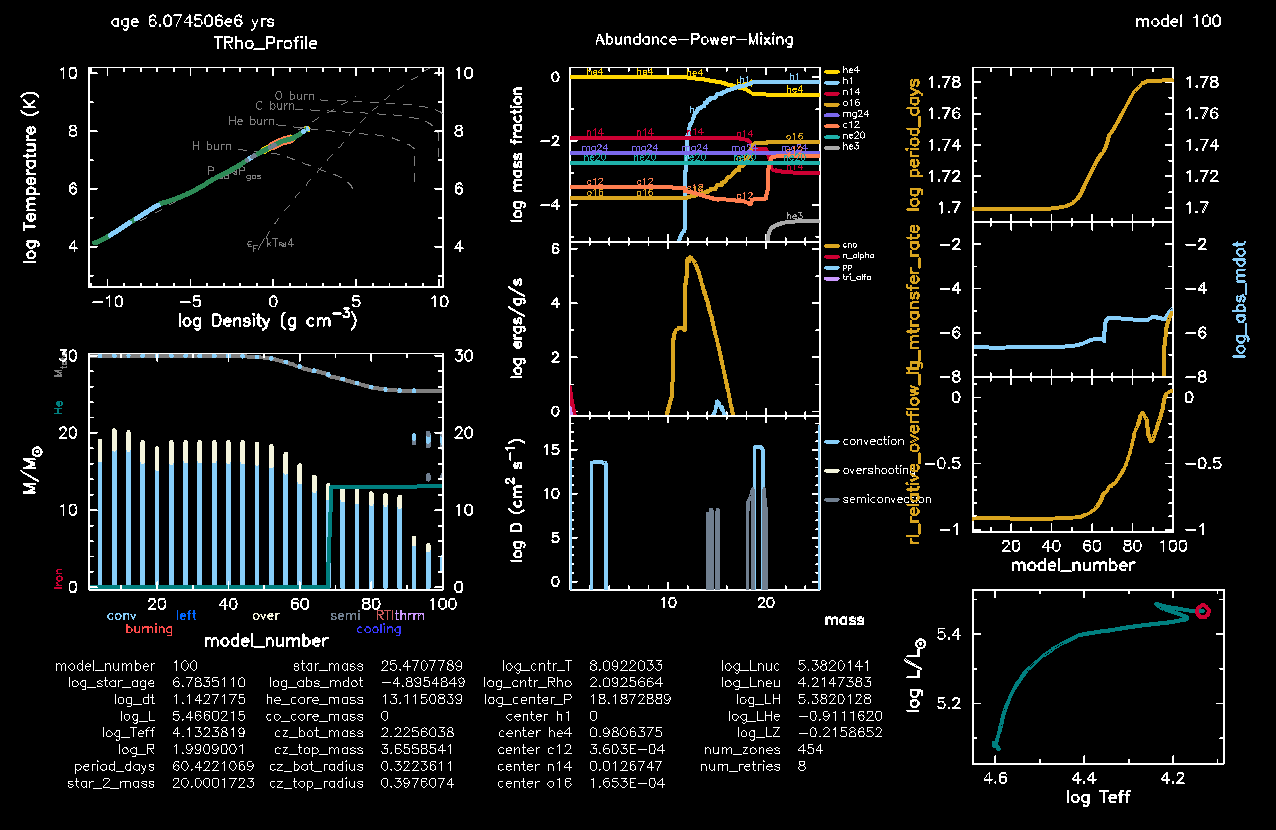
Owing to its long period orbit, this system undergoes Roche lobe overflow right after the main sequence. The objective of this minilab is to time how long this phase lasts, and what impact it has on the orbit. The questions you have to answer are the following:
How long does the Roche lobe overflow phase last? How does this compare to the total lifestyle of the system?
How does the orbital period respond to mass transfer?
What are the properties of the donor after the mass transfer phase?
How does the mass transfer rate compare to the Eddington rate of the black hole?
How do the results change depending on the prescription used for mass transfer?
Instructions on how to time the Roche lobe overflow phase, as well as how to change mass transfer prescription, are given in the next subsections.
To time the phase of Roche lobe overflow, we will add code in the extras_binary_check_model subroutine of run_binary_extras. A few pointers on how to do this follow:
The radius and roche lobe radius of the star can be accesed through b% r(1) and b% rl(1).
The timestep in years can be accesed with b% time_step.
You can make use of b% xtra(1) to keep track of the total time in Roche lobe overflow. As mentioned previously, b% xtra is available for users to store information, and the code internally takes care of adjusting it in case of retries, as well as restoring it during a restart. At the start of the simulation all values of b% xtra are set to zero.
For simplicity, you can just print the age to the terminal using write(*,*) "check time", b% xtra(1).
extras_binary_finish_step, but owing to a bug in the latest release, changes to b% xtra done in this subroutine are not properly stored.Are you having trouble implementing this? Compare your work with that of your neighbouring students and TA. If you still have problems finding a solution, you can check an implementation of this by clicking the box below.
integer function extras_binary_check_model(binary_id)
   type (binary_info), pointer :: b
   integer, intent(in) :: binary_id
   integer :: ierr
   call binary_ptr(binary_id, b, ierr)
   if (ierr /= 0) then ! failure in  binary_ptr
      return
   end if
   extras_binary_check_model = keep_going

   if (b% r(1) > b% rl(1)) then
       b% xtra(1) = b% xtra(1)+b% time_step
   end if
   write(*,*) "check time", b% xtra(1)

end function extras_binary_check_modelThe mass transfer prescription, referred in MESA by the option mdot_scheme, is an important aspect that should be taken into account when modelling binaries. It is also one you must remember to acknowledge when publishing work done with MESA, by specifying the prescription used and citing the corresponding source. As we are not doing 3D hydrodynamics, we need to rely in approximations that determine the mass transfer rate given the current state of the binary system. To adjust the prescription you can use the following in the @binary_controls section of inlist_project:
mdot_scheme = 'Ritter'The main mass transfer schemes available are:
roche_lobe: Mass transfer rate is determined such that the surface of the donor star remains within its roche lobe.
Ritter: Follows Ritter (1988) to account for mass transfer through L1 from an extended atmosphere before the onset of Roche lobe overflow. This is the default option.
Kolb: Follows Kolb & Ritter(1990), and extension of the Ritter scheme that accounts for the effect of overflow from regions below the photosphere.
You should perform two runs, using the Ritter and the Kolb schemes. Provide answers to the questions for both. Depending on time, you might want to split work across others in your table. For example, two people can do the run with Ritter while the other two do the run with Kolb. This can be useful to validate your results.
Have you finished early? Then congrats! I also don't want you just hovering around, so you can do the following:
See how the outcome of binary interaction is modified for a different orbital period. For example, consider periods of and days. Is the final product of binary evolution significantly different?
In computing the time during which the system undergoes mass transfer we have ignored a small detail. When the system enters into Roche lobe overflow and detaches, it will do so only for a fraction of the timestep. The provided solution ignores this subtlety and includes the entire timestep. How would you correct for this?
de Jager, C., Nieuwenhuijzen, H., van der Hucht, K. A., Astronomy and Astrophysics, Suppl. Ser., Vol. 72, p. 259-289 (1988)
Ritter, H.,, Astronomy and Astrophysics, Vol. 202, p. 93-100 (1988)
Kolb, U., Ritter, H.,, Astronomy and Astrophysics, Vol. 236, p. 385-392 (1990)
Nugis, T., Lamers, H. J. G. L. M., Astronomy and Astrophysics, Vol. 360, p.227-244 (2000)
Vink, Jorick S., de Koter, A., Lamers, H. J. G. L. M., Astronomy and Astrophysics, v.369, p.574-588 (2001)
Brott, I., de Mink, S. E., Cantiello, M., Langer, N., de Koter, A., Evans, C. J., Hunter, I., Trundle, C., Vink, J. S., Astronomy & Astrophysics, Volume 530, id.A115, 20 pp. (2011)